Description

This project was declared by one of our university’s teachers, who taught us a course called ‘Basic of Data Mining’. To do this project, we had to choose a dataset and, consequently, divide the project into 4 sections and do each of them one by one.

First section: Dataset

The downloaded dataset for my project was Covid-19 statistics in Italy from 24/02/2022 to 15/06/2022 from Kaggle. I preferred to choose this dataset because of two main reasons:

1. My mother is a nurse, so unconsciously, I have dealt with Covid-19 and its difficulties from the first days of the pandemic.
2. I have liked Italy since childhood since I watched some movies and played some video games made in Italy.

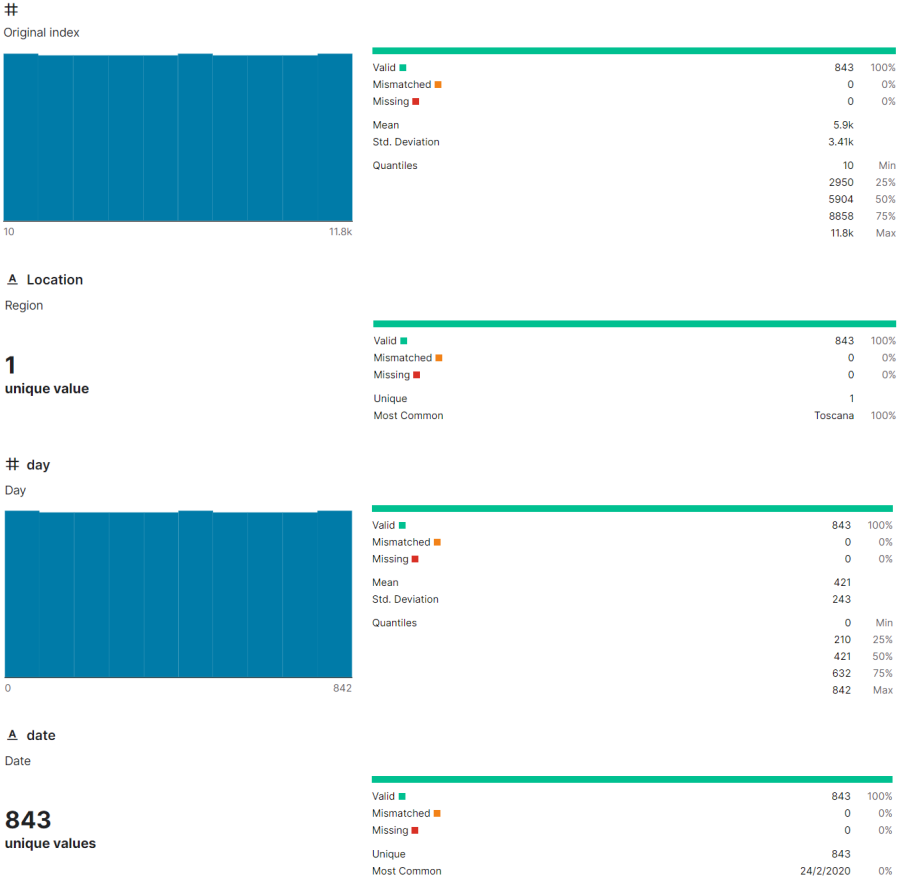
This chosen dataset has 13 rows and 844 columns, and these attributes’ information is listed in the below section:

• original_index: Numeric
• location: Nominal
• day: Numeric
• date: Nominal
• total_number_positive_people: Numeric
• deaths: Numeric
• deaths_increase: Numeric
• total_recoveries: Numeric
• total_recoveries_increase: Numeric
• currently_positive: Numeric
• dismissed_patients: Numeric
• swabs: Numeric
• swabs_increase: Numeric

Also, the dataset format was ‘CSV’, an Excell file.

The dataset author provides some information in Kaggle:

Second section: Data Preprocessing

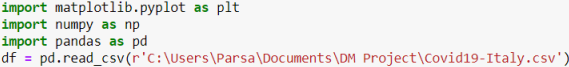
In this step, I import important libraries for loading my dataset and drawing plots.

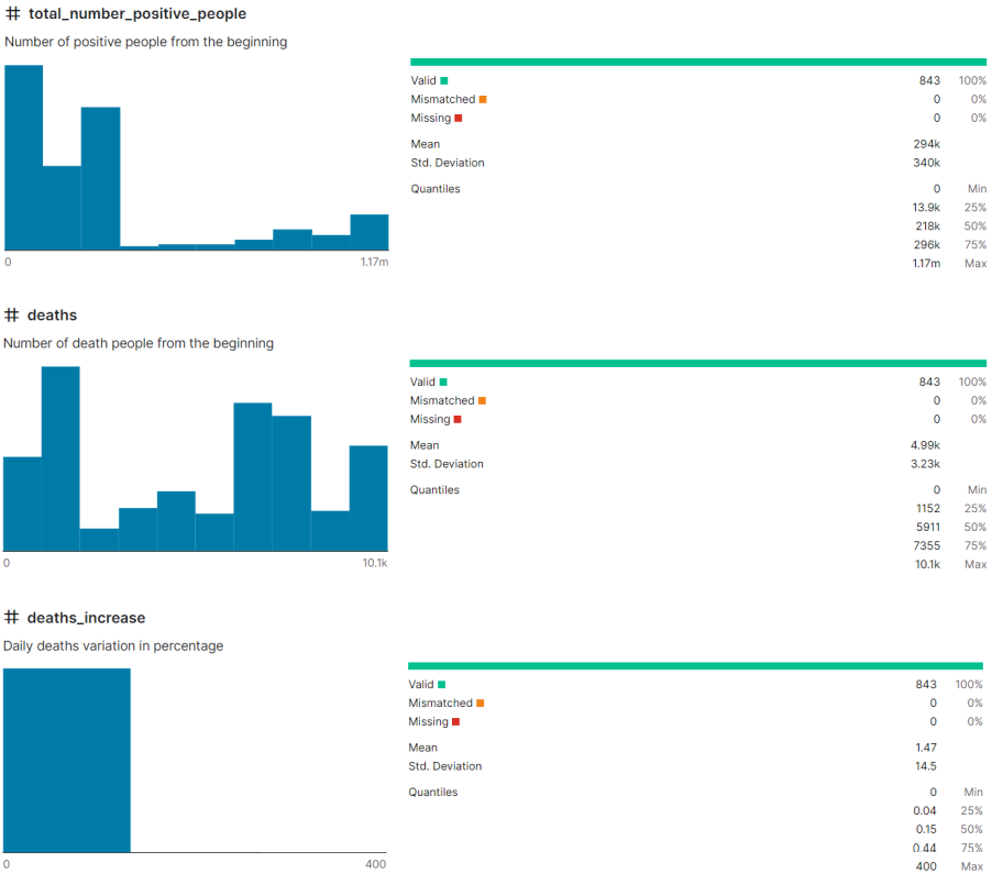
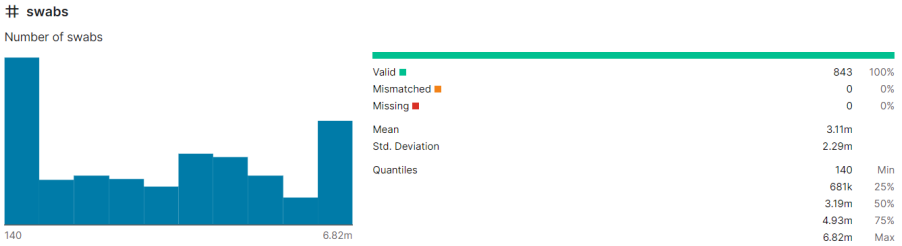
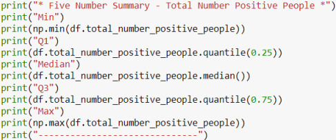
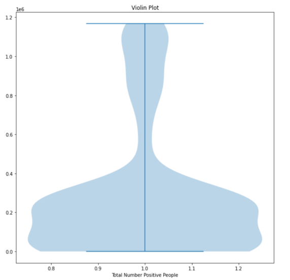
In the next step, I calculated 5 number summary for the total_number_positive_people attribute:

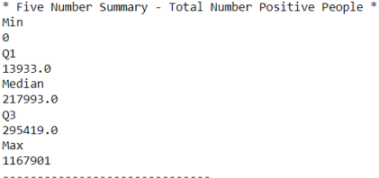
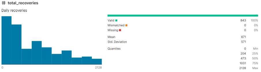
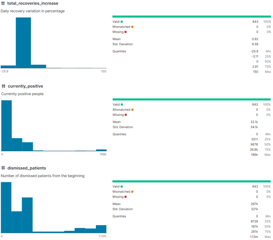
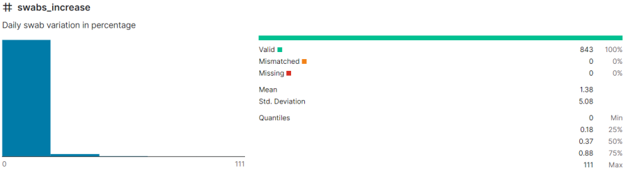
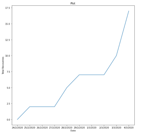
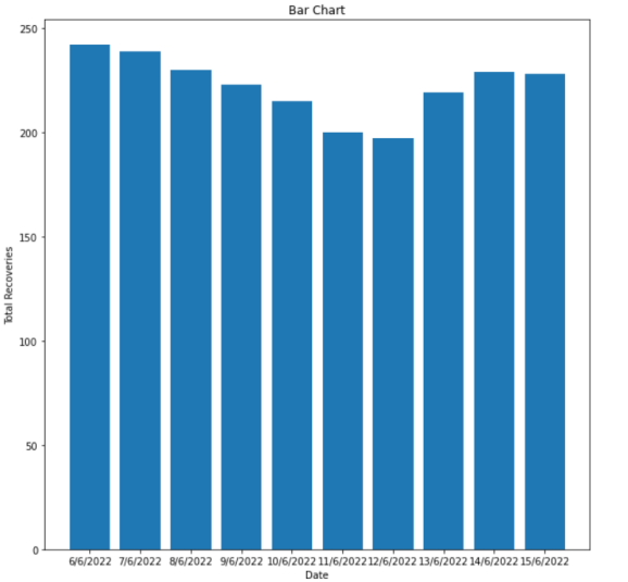
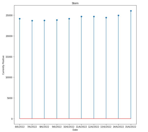
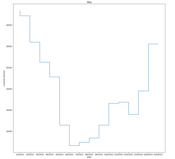
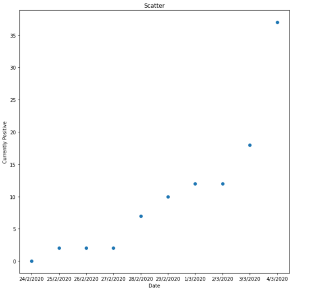
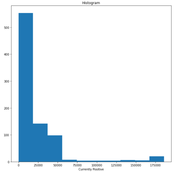
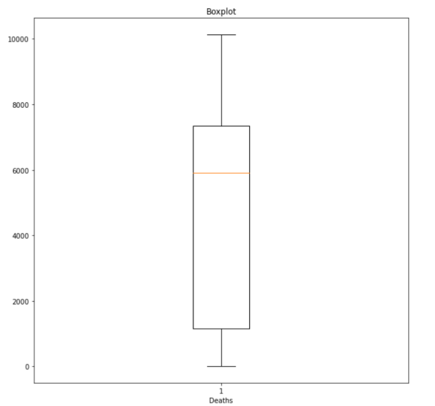
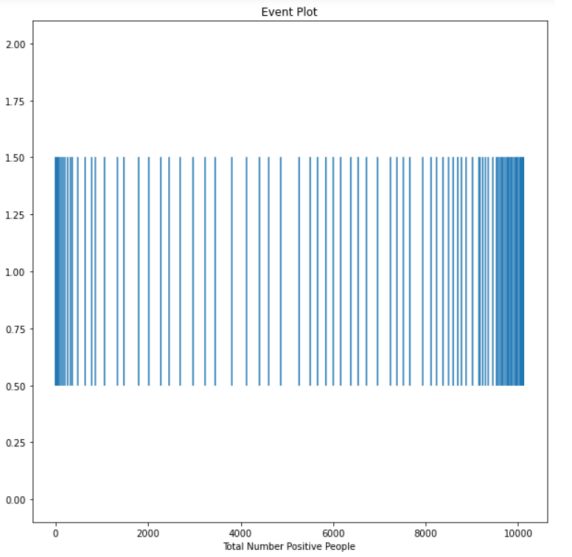
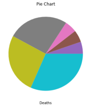
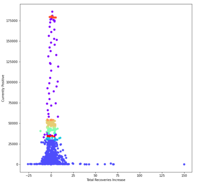
I also do the same thing for other attributes. Anyway, then I draw ten different plots for my dataset:

Third section: Clustering

In this section, I used four different methods:

1. K-means
2. K-medoids
3. Hierarchical (Agglomerative)
4. Density (DBScan)

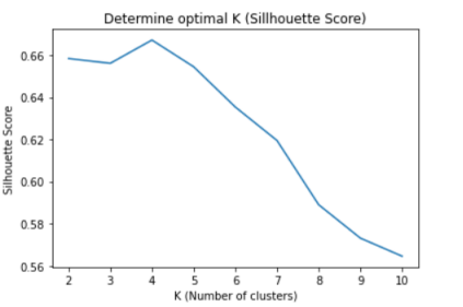
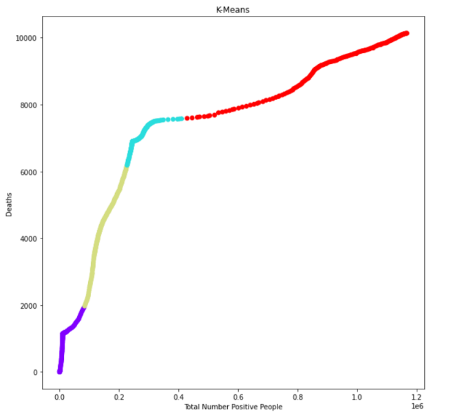
1- K-means:

Firstly, I used the silhouette score to find the optimal k for clustering, which is four at this moment:

Then, I wrote some lines of code, and the output was:

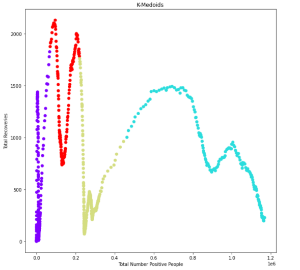
2- K-medoids:

In this part, I wrote my code, but I found out that I needed to install the sklearn_extra.cluster from Powershell prompt, so I did this:

After installing the mentioned library, I executed my code, and this is the output that I got:

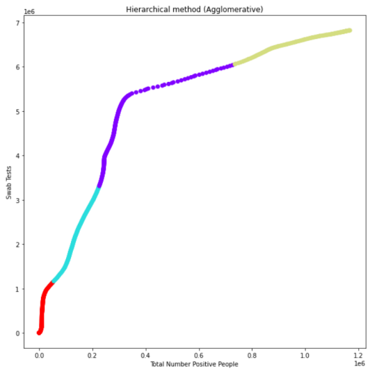
3- Hierarchical (Agglomerative):

In this method, I used the Euclidean method to calculate distances. The output:

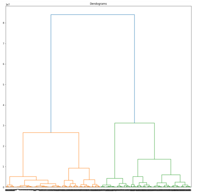
Then, I draw a dendrogram diagram:

4- Density (DBScan):

After writing this part’s code, the exported output is (min_samples: 4, eps = 500):

Fourth section: Classification

In this part, I used two methods:

1. Information Gain (ID3)
2. Naive Bayes

1- Information Gain (ID3):

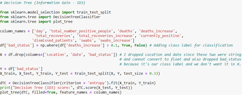
This part of the code is related to the information gain method, and there is a score which is printed in the last part of the code:

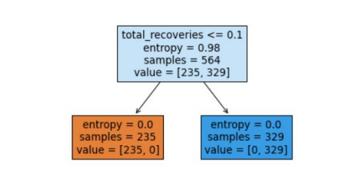
And in the last line, I wrote plot_tree(dTC, filled=True, feature_names = column_names) which means the program will draw a tree for us:

2- Naive Bayes:

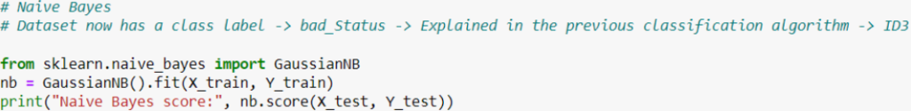
By using this method, the given score is:

After comparing these two scores, it is evident that the second one is more precise.